CF-FM call segmentation accuracy

This page will illustrate the accuracy with which itsfm can segment CF-FM parts of a CF-FM call. To see what a CF-FM call looks like check out the bat-call example in the ‘Basic Examples’ page.

The synthetic data has already been generated and run with the segment_and_measure function, and now we’ll compare the accuracy with which it has all happened.

A CF-FM bat call typically has three parts to it, 1) an ‘up’ FM, where the frequency of the call increases, 2) a ‘CF’ part, where the frequency is stable, and then 3) a ‘down’ FM, where the frequency drops. The synthetic data is basically a set of CF-FM calls with a combination of upFM, downFM and CF part durations, bandwidths,etc.

Here we will only be seeing if the durations of each of the segment parts have been picked up properly or not. We will not be performing any accuracy assessments on the exact parameters (eg. peak frequency, rms, etc) because it is assumed that if the call parts can be identified by their durations then the measurements will in turn be as expected.

There is no silence in the synthetic calls, and no noise too. This is the situation which should provide the highest accuracy.

What happened before

To see more on the details of the generation and running of the synthetic data see the modules CF/FM call segmentation and Generating the CF-FM synthetic calls

import itsfm
import matplotlib.pyplot as plt
plt.rcParams['agg.path.chunksize'] = 10000
import numpy as np
import pandas as pd
import seaborn as sns
import tqdm

obtained = pd.read_csv('obtained_pwvd_horseshoe_sim.csv')
synthesised = pd.read_csv('horseshoe_test_parameters.csv')

Let’s look at the obtained regions and their durations

obtained

We can see the output has each CF/FM region labelled by the order in which they’re found. Let’s re-label these to match the names of the synthesised call parameter dataframe. ‘upfm’ is fm1, ‘downfm’ is fm2.

obtained.columns = ['call_number','cf_duration',
                    'upfm_duration', 'downfm_duration', 'other']

Let’s look at the synthetic call parameters. There’s a bunch of parameters that’re not interesting for this accuracy exercise and so let’s remove them

synthesised

synthesised.columns

synth_regions = synthesised.loc[:,['cf_duration', 'upfm_duration','downfm_duration']]
synth_regions['other'] = np.nan
synth_regions['call_number'] = obtained['call_number']

Comparing the synthetic and the obtained results

We have the two datasets formatted properly, now let’s compare the accuracy of itsfm.

accuracy = obtained/synth_regions
accuracy['call_number'] = obtained['call_number']

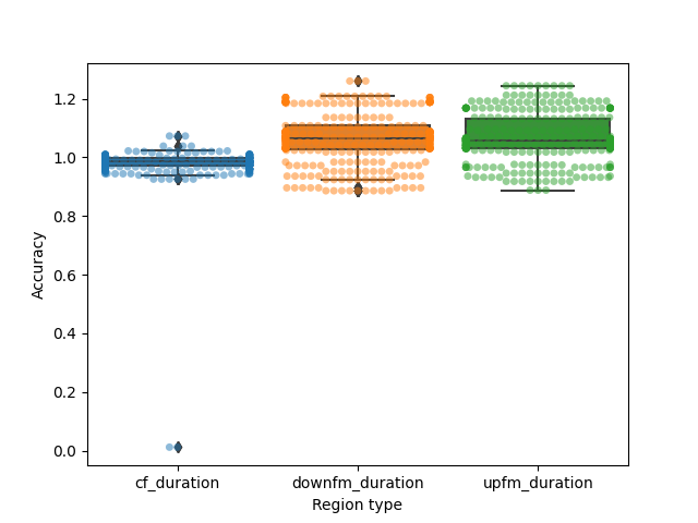
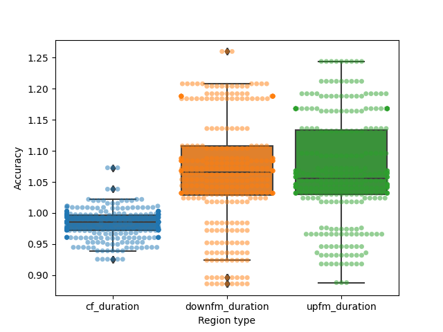
Overall accuracy of segmentation:

accuracy_reformat = accuracy.melt(id_vars=['call_number'],
                                            var_name='Region type',
                                            value_name='Accuracy')

accuracy_reformat = accuracy_reformat[accuracy_reformat['Region type']!='other']

plt.figure()

ax = sns.boxplot(x='Region type', y = 'Accuracy',
                         data=accuracy_reformat)

ax = sns.swarmplot(x='Region type', y = 'Accuracy',
                         data=accuracy_reformat,
                         alpha=0.5)

Out:

/home/docs/checkouts/readthedocs.org/user_builds/itsfm/envs/latest/lib/python3.7/site-packages/seaborn/categorical.py:1296: UserWarning: 75.3% of the points cannot be placed; you may want to decrease the size of the markers or use stripplot.
  warnings.warn(msg, UserWarning)
/home/docs/checkouts/readthedocs.org/user_builds/itsfm/envs/latest/lib/python3.7/site-packages/seaborn/categorical.py:1296: UserWarning: 46.0% of the points cannot be placed; you may want to decrease the size of the markers or use stripplot.
  warnings.warn(msg, UserWarning)
/home/docs/checkouts/readthedocs.org/user_builds/itsfm/envs/latest/lib/python3.7/site-packages/seaborn/categorical.py:1296: UserWarning: 40.7% of the points cannot be placed; you may want to decrease the size of the markers or use stripplot.
  warnings.warn(msg, UserWarning)

Peak-percentage method accuracy

Now let’s take a look at the peak percentage method’s accuracy

obtained_pkpct = pd.read_csv('obtained_pkpct_horseshoe_sim.csv')

obtained_pkpct.head()

It can clearly be seen that there are some calls with multiple segments detected. This multiplicity of segments typically results from false positive detections, where the CF-FM ratio jumps above 0 spuriously for a few samples. Let’s take a look at some of these situations.

def identify_valid_segmentations(df):
    '''
    Identifies if a segmentation output has valid (numeric)
    entries for cf1, fm1, fm2, and NaN for all other columns.

    Parameters
    ----------
    df : pd.DataFrame
        with at least the following column names, 'cf1','fm1','fm2'

    Returns
    -------
    valid_segmentation: bool.
        True, if the segmentation is valid.
    '''
    all_columns = df.columns
    target_columns = ['cf1','fm1','fm2']
    rest_columns = set(all_columns)-set(target_columns)
    rest_columns = rest_columns - set(['call_number'])

    valid_cf1fm1fm2 = lambda row, target_columns: np.all([ ~np.isnan(row[each]) for each in target_columns])
    all_otherrows_nan = lambda row, rest_columns: np.all([ np.isnan(row[each]) for each in rest_columns])

    all_valid_rows = np.zeros(df.shape[0],dtype=bool)
    for i, row in df.iterrows():
        all_valid_rows[i] = np.all([valid_cf1fm1fm2(row, target_columns),
                                          all_otherrows_nan(row, rest_columns)])
    return all_valid_rows

calls_w_3segs = identify_valid_segmentations(obtained_pkpct)

print(f'{np.sum(calls_w_3segs)/calls_w_3segs.size} % of calls have 3 segments')

Out:

0.9444444444444444 % of calls have 3 segments

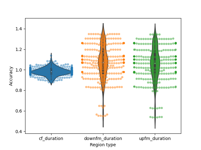
6% of calls don’t have 3 components - let’s remove these poorly segmented calls and quantify their segmentation accuracy.

pkpct_well_segmented = obtained_pkpct.loc[calls_w_3segs,:]
pkpct_well_segmented = pkpct_well_segmented.drop(['cf2','fm3','fm4'],axis=1)

pkpct_well_segmented.columns = ['call_number','cf_duration',
                    'upfm_duration', 'downfm_duration', 'other']

pkpct_accuracy = pkpct_well_segmented/synth_regions.loc[calls_w_3segs,:]


# Overall accuracy of segmentation:
pkpct_accuracy_reformat = pkpct_accuracy.melt(id_vars=['call_number'],
                                            var_name='Region type',
                                            value_name='Accuracy')
pkpct_accuracy_reformat = pkpct_accuracy_reformat[pkpct_accuracy_reformat['Region type']!='other']

plt.figure()
ax = sns.violinplot(x='Region type', y = 'Accuracy',
                         data=pkpct_accuracy_reformat)

ax = sns.swarmplot(x='Region type', y = 'Accuracy',
                         data=pkpct_accuracy_reformat,
                         alpha=0.5)

Out:

/home/docs/checkouts/readthedocs.org/user_builds/itsfm/envs/latest/lib/python3.7/site-packages/seaborn/categorical.py:1296: UserWarning: 51.6% of the points cannot be placed; you may want to decrease the size of the markers or use stripplot.
  warnings.warn(msg, UserWarning)
/home/docs/checkouts/readthedocs.org/user_builds/itsfm/envs/latest/lib/python3.7/site-packages/seaborn/categorical.py:1296: UserWarning: 19.0% of the points cannot be placed; you may want to decrease the size of the markers or use stripplot.
  warnings.warn(msg, UserWarning)
/home/docs/checkouts/readthedocs.org/user_builds/itsfm/envs/latest/lib/python3.7/site-packages/seaborn/categorical.py:1296: UserWarning: 26.8% of the points cannot be placed; you may want to decrease the size of the markers or use stripplot.
  warnings.warn(msg, UserWarning)

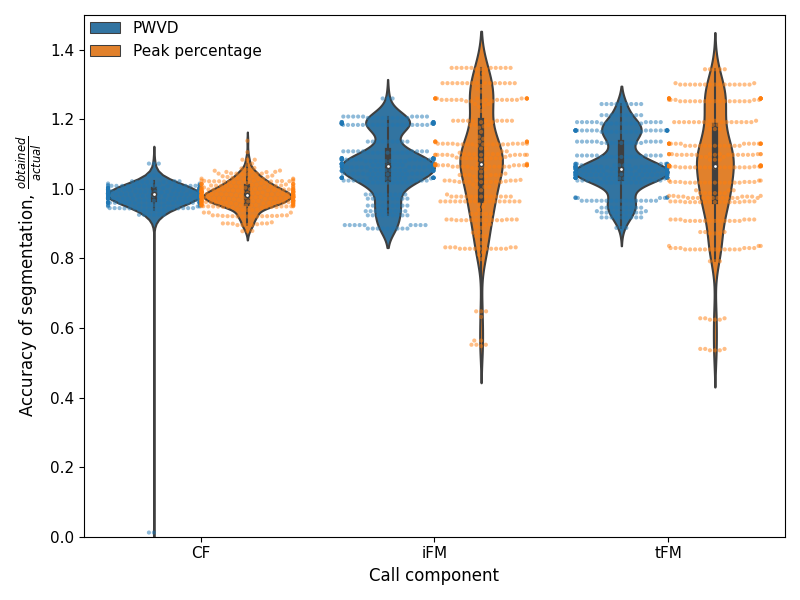
Putting it all together: PWVD vs peak percentage

pwvd_accuracy = accuracy_reformat.copy()
pwvd_accuracy['method'] = 'pwvd'

pkpct_accuracy = pkpct_accuracy_reformat.copy()
pkpct_accuracy['method'] = 'pkpct'


both_accuracy = pd.concat([pwvd_accuracy, pkpct_accuracy])
both_accuracy['combined_id'] = both_accuracy['Region type']+both_accuracy['method']


grouped_accuracy = both_accuracy.groupby(['Region type','method'])

plt.figure(figsize=(8,6))
ax = sns.swarmplot(x='Region type', y = 'Accuracy',
                         data=both_accuracy, hue='method',hue_order=["pwvd", "pkpct"],
                         dodge=True,alpha=0.5, s=3)

ax2 = sns.violinplot(x='Region type', y = 'Accuracy',
                         data=both_accuracy, hue='method',hue_order=["pwvd", "pkpct"],
                         dodge=True,alpha=0.5, s=2.5)
ax2.legend_.remove()
handles, labels = ax2.get_legend_handles_labels() # thanks Ffisegydd@ https://stackoverflow.com/a/35539098
l = plt.legend(handles[0:2], ['PWVD','Peak percentage'], loc=2, fontsize=11,
               borderaxespad=0., frameon=False)

plt.xticks([0,1,2],['CF','iFM','tFM'], fontsize=11)
plt.xlabel('Call component',fontsize=12);plt.ylabel('Accuracy of segmentation, $\\frac{obtained}{actual}$',fontsize=12);
plt.yticks(fontsize=11)
plt.ylim(0,1.5)
plt.tight_layout()
plt.savefig('pwvd-pkpct-comparison.png')

Out:

/home/docs/checkouts/readthedocs.org/user_builds/itsfm/envs/latest/lib/python3.7/site-packages/seaborn/categorical.py:1296: UserWarning: 60.5% of the points cannot be placed; you may want to decrease the size of the markers or use stripplot.
  warnings.warn(msg, UserWarning)
/home/docs/checkouts/readthedocs.org/user_builds/itsfm/envs/latest/lib/python3.7/site-packages/seaborn/categorical.py:1296: UserWarning: 37.3% of the points cannot be placed; you may want to decrease the size of the markers or use stripplot.
  warnings.warn(msg, UserWarning)
/home/docs/checkouts/readthedocs.org/user_builds/itsfm/envs/latest/lib/python3.7/site-packages/seaborn/categorical.py:1296: UserWarning: 32.1% of the points cannot be placed; you may want to decrease the size of the markers or use stripplot.
  warnings.warn(msg, UserWarning)
/home/docs/checkouts/readthedocs.org/user_builds/itsfm/envs/latest/lib/python3.7/site-packages/seaborn/categorical.py:1296: UserWarning: 11.1% of the points cannot be placed; you may want to decrease the size of the markers or use stripplot.
  warnings.warn(msg, UserWarning)
/home/docs/checkouts/readthedocs.org/user_builds/itsfm/envs/latest/lib/python3.7/site-packages/seaborn/categorical.py:1296: UserWarning: 31.2% of the points cannot be placed; you may want to decrease the size of the markers or use stripplot.
  warnings.warn(msg, UserWarning)
/home/docs/checkouts/readthedocs.org/user_builds/itsfm/envs/latest/lib/python3.7/site-packages/seaborn/categorical.py:1296: UserWarning: 19.6% of the points cannot be placed; you may want to decrease the size of the markers or use stripplot.
  warnings.warn(msg, UserWarning)

What are the 95%ile limits of the accuracy?

accuracy_ranges = grouped_accuracy.apply(lambda X: np.nanpercentile(X['Accuracy'],[2.5,97.5]))
accuracy_ranges

Out:

Region type      method
cf_duration      pkpct                [0.8994, 1.05945]
                 pwvd      [0.9392, 1.0218500000000001]
downfm_duration  pkpct                   [0.648, 1.348]
                 pwvd       [0.8867499999999999, 1.208]
upfm_duration    pkpct      [0.624, 1.2999999999999998]
                 pwvd      [0.9179999999999999, 1.2416]
dtype: object

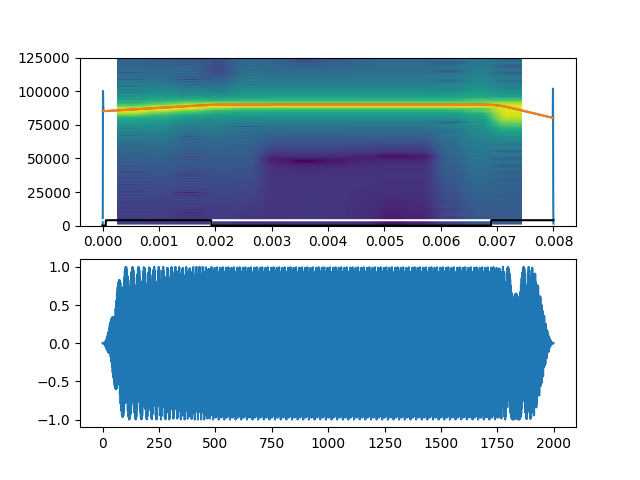
Troubleshooting the ‘bad’ fixes - what went wrong?

Some bad PWVD identifications

As we can see there are a few regions where the accuracy is very low, let’s investigate which of these calls are doing badly.

poor_msmts = accuracy[accuracy['cf_duration']<0.5].index

Now, let’s troubleshooot this particular set of poor measurements fully.

simcall_params = pd.read_csv('horseshoe_test_parameters.csv')
obtained_params = pd.read_csv('obtained_pwvd_horseshoe_sim.csv')

obtained_params.loc[poor_msmts,:]

There are two CF regions being recognised, one of them is just extremely short. Where is this coming from? Let’s take a look at the actual frequency tracking output, by re-running the `itsfm` routine once more:

import h5py


f = h5py.File('horseshoe_test.hdf5', 'r')

fs = float(f['fs'][:])

parameters = {}
parameters['segment_method'] = 'pwvd'
parameters['window_size'] = int(fs*0.001)
parameters['fmrate_threshold'] = 2.0
parameters['max_acc'] = 10
parameters['extrap_window'] = 75*10**-6

raw_audio = {}

for call_num in tqdm.tqdm(poor_msmts.to_list()):
    synthetic_call = f[str(call_num)][:]
    raw_audio[str(call_num)] = synthetic_call
    output = itsfm.segment_and_measure_call(synthetic_call, fs, **parameters)

    seg_output, call_parts, measurements= output

    # # save the long format output into a wide format output to
    # # allow comparison
    # sub = measurements[['region_id', 'duration']]
    # sub['call_number'] = call_num
    # region_durations = sub.pivot(index='call_number',
    #                              columns='region_id', values='duration')
    # obtained.append(region_durations)

f.close()

call_num = str(poor_msmts[0])

plt.figure()
plt.subplot(211)
plt.specgram(raw_audio[call_num], Fs=fs)
plt.plot(np.linspace(0,raw_audio[call_num].size/fs,raw_audio[call_num].size),
         seg_output[2]['raw_fp'])
plt.plot(np.linspace(0,raw_audio[call_num].size/fs,raw_audio[call_num].size),
         seg_output[2]['fitted_fp'])
plt.plot(np.linspace(0,raw_audio[call_num].size/fs,raw_audio[call_num].size),
         seg_output[0]*4000,'w')
plt.plot(np.linspace(0,raw_audio[call_num].size/fs,raw_audio[call_num].size),
         seg_output[1]*4000,'k')
plt.subplot(212)
plt.plot(raw_audio[call_num])

plt.figure()
plt.subplot(311)
plt.plot(np.linspace(0,raw_audio[call_num].size/fs,raw_audio[call_num].size),
         seg_output[2]['raw_fp'])
plt.subplot(312)
plt.plot(np.linspace(0,raw_audio[call_num].size/fs,raw_audio[call_num].size),
         seg_output[2]['fmrate'])
#plt.plot(np.linspace(0,raw_audio[call_num].size/fs,raw_audio[call_num].size),
#         seg_output[0]*5,'k',label='CF')
#plt.plot(np.linspace(0,raw_audio[call_num].size/fs,raw_audio[call_num].size),
#         seg_output[1]*5,'r', label='FM')
plt.hlines(2, 0, raw_audio[call_num].size/fs, linestyle='dotted', alpha=0.5,
           label='2kHz/ms fm rate')
plt.legend()
plt.subplot(313)
plt.plot(raw_audio[call_num])

• 
• 

Out:

  0%|          | 0/2 [00:00<?, ?it/s]
 50%|#####     | 1/2 [00:01<00:01,  1.01s/it]
100%|##########| 2/2 [00:02<00:00,  1.01s/it]
100%|##########| 2/2 [00:02<00:00,  1.01s/it]

[<matplotlib.lines.Line2D object at 0x7f40e96ac190>]

Making some corrections to the PWVD output

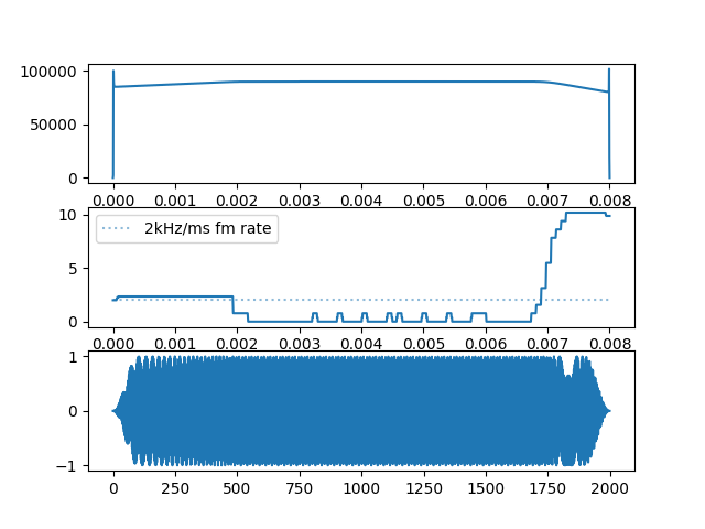
Here, we can see that the ‘error’ is that the FM rate is very slightly below the 2 kHz/ms FM rate, and thus appears as a false CF region. This slight drop in FM rate is also because of edge effects. The frequency profile correction methods in place were able to recognise the odd spike in frequency profile and interpolate between two regions with reliable frequency profiles. This interpolation thus lead to a slight drop in the FM rate.

Considering that the CF measurement is actually there, but labelled as CF2, let’s correct this labelling error and then see the final accuracy. We will not attempt to compensate for this error by adjusting the iFM duration here.

corrected_obtained = obtained_params.copy()
for each in poor_msmts:
    corrected_obtained.loc[each,'cf1'] = corrected_obtained.loc[each,'cf2']
    corrected_obtained.loc[each,'other'] = np.nan

corrected_obtained = corrected_obtained.loc[:,corrected_obtained.columns!='cf2']

corrected_obtained.columns = ['call_number','cf_duration',
                    'upfm_duration', 'downfm_duration', 'other']

corrected_accuracy = corrected_obtained/synth_regions
corrected_accuracy['call_number'] = corrected_obtained['call_number']
corrected_accuracy_reformat = corrected_accuracy.melt(id_vars=['call_number'],
                                            var_name='Region type',
                                            value_name='Accuracy')
corrected_accuracy_reformat = corrected_accuracy_reformat.loc[corrected_accuracy_reformat['Region type']!='other',:]

plt.figure()
ax = sns.boxplot(x='Region type', y = 'Accuracy',
                         data=corrected_accuracy_reformat)

ax = sns.swarmplot(x='Region type', y = 'Accuracy',
                         data=corrected_accuracy_reformat,
                         alpha=0.5)

Out:

/home/docs/checkouts/readthedocs.org/user_builds/itsfm/envs/latest/lib/python3.7/site-packages/seaborn/categorical.py:1296: UserWarning: 47.8% of the points cannot be placed; you may want to decrease the size of the markers or use stripplot.
  warnings.warn(msg, UserWarning)
/home/docs/checkouts/readthedocs.org/user_builds/itsfm/envs/latest/lib/python3.7/site-packages/seaborn/categorical.py:1296: UserWarning: 14.5% of the points cannot be placed; you may want to decrease the size of the markers or use stripplot.
  warnings.warn(msg, UserWarning)
/home/docs/checkouts/readthedocs.org/user_builds/itsfm/envs/latest/lib/python3.7/site-packages/seaborn/categorical.py:1296: UserWarning: 19.8% of the points cannot be placed; you may want to decrease the size of the markers or use stripplot.
  warnings.warn(msg, UserWarning)