‘Difficult’ example

The <insertname> package was mainly designed keeping horseshoe bat calls in mind. These calls are high-frequency (>50kHz) and short (20-50ms) sounds which are quite unique in their structure. Many of the default parameter values reflect the original dataset. In fact, many of the default parameters don’t even work for some of the example datasets themselves! It should be no surprise that unpredictable things happen when segmentation and tracking is run with default values.

This example will guide you through understanding the various parameters that can be tweaked and what effect they actually have. It is not an exhaustive treatment of the implementation, but a ‘lite’ intro. For more details of course, the original documentation should hopefully be helpful.

from matplotlib.lines import Line2D
import matplotlib.pyplot as plt
import itsfm
from itsfm.data import example_calls, all_wav_files

# a chosen set of tricky calls to illustrate various points

tricky_rec = list(map( lambda X: '2018-08-17_23_115' in X, all_wav_files))
index = tricky_rec.index(True)
audio, fs = example_calls[index] # load the relevant example audio

Step 1: the right signal_level

In the given audio segment, the first step is to identify what is background and what is signal. The signal of interest is identified as being above a particular dB rms, as calculated y a moving dB rms window of a user-defined window_size.

If we want high temporal resolution to segment out the call, we need a short window_size. Let’s try out 0.5 and 2ms for now.

halfms_windowsize = int(fs*0.5*10**-3)
twoms_windowsize = halfms_windowsize*4
plt.figure()
ax = plt.subplot(211)
itsfm.plot_movingdbrms(audio, fs, window_size=halfms_windowsize)
itsfm.plot_movingdbrms(audio, fs, window_size=twoms_windowsize)

first_color = '#1f77b4'
second_color = '#ff7f0e'
custom_lines = [Line2D([0],[0], color=first_color),
                Line2D([1],[1],color=second_color),]
ax.legend(custom_lines, ['0.5ms', '2ms'])
plt.ylabel('Moving dB rms')
plt.subplot(212, sharex=ax)
_ = itsfm.make_specgram(audio, fs);

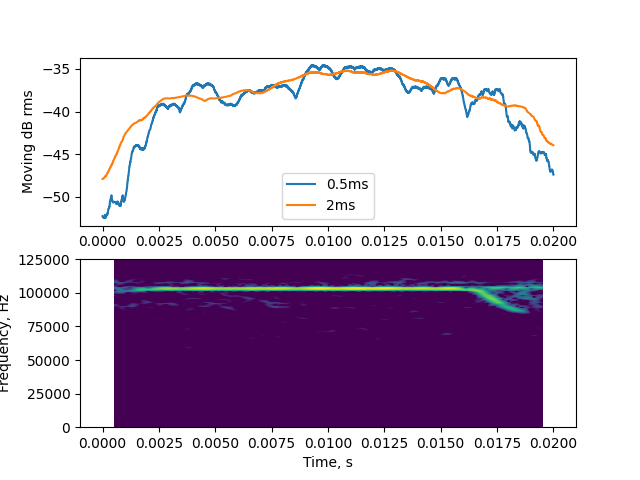
The fact that the 0.5ms moving rms profile is so ‘rough’ is already a bad sign. The signal of interest is any region/s which are above or equal to the signal_level. When the moving rms fluctuates so wildly, the relevant signal region may be hard to capture because it keeps going above and below the threshold - leading to many tiny ‘íslands’. Let’s choose the 2ms window_size because it doesn’t fluctuate crazily and is also a relatively short time scale in comparison the the signal duration. -40 dB rms seems to be a sensible value when we compare the approximate start and end times of the signal with the dB rms profile.

keywords = {'segment_method':'pwvd',
            'signal_level':-40,
            'window_size':twoms_windowsize}

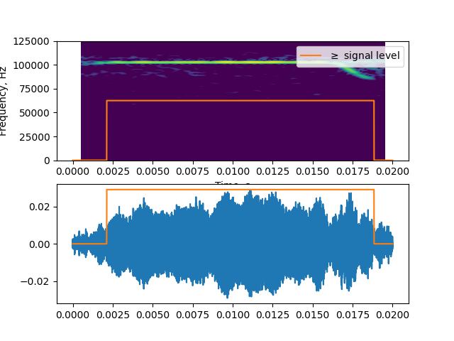
outputs = itsfm.segment_and_measure_call(audio, fs,**keywords)
output_inspector = itsfm.itsFMInspector(outputs, audio, fs)

output_inspector.visualise_geq_signallevel()

Out:

(<AxesSubplot:xlabel='Time, s', ylabel='Frequency, Hz'>, <AxesSubplot:>)

Let’s check the output as it is right now

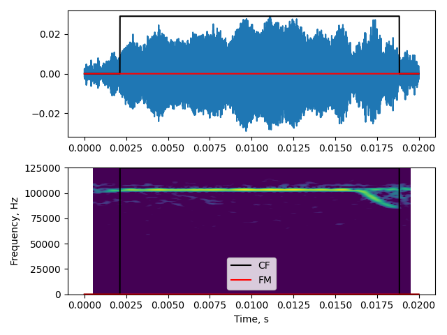
output_inspector.visualise_cffm_segmentation()

Out:

(<AxesSubplot:>, <AxesSubplot:xlabel='Time, s', ylabel='Frequency, Hz'>)

Inspect initial outputs The CF-FM segmentation is clearly not correct. There’s FM component recognised at all - how is this happening? The reason it’s not happening is likely because the fmrate has been misspecified or the frequency profile wasn’t estimated correctly. Let’s view the frequency profile first.

output_inspector.visualise_frequency_profiles()

Out:

(<AxesSubplot:xlabel='Time, s', ylabel='Frequency, Hz'>, <AxesSubplot:>)

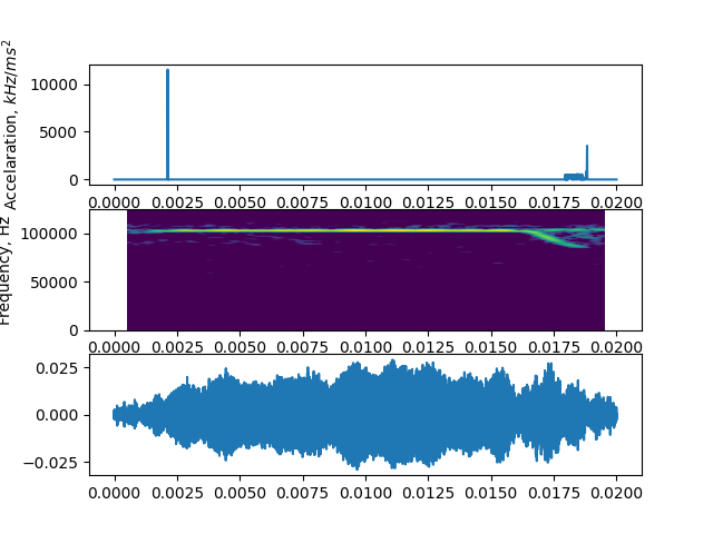
The cleaned frequency profile seems to somehow ‘ignore’ the downward FM sweep in the call. Why is this happening? The ‘flatness’ in the cleaned frequency profile is likely coming from the spike detection. Spikes in the frequency profile are detected when the ‘accelaration’ of (the 2nd derivative) the frequency profile increases beyond a threshold. Let’s check out the accelaration profile

output_inspector.visualise_accelaration()

Out:

(<AxesSubplot:ylabel='Accelaration, $kHz/ms^{2}$'>, <AxesSubplot:xlabel='Time, s', ylabel='Frequency, Hz'>, <AxesSubplot:>)

The accelaration profile matches this suspicion. When a spikey region is encountered in the frequency profile in the pwvd frequency tracking - it backs up a bit and extrapolates the slope according to what’s just behind the spikey region. The ‘length’ of this backing up in seconds is decided by the extrap_window, which is short for extrapolation window. Let’s reduce the extrap_window and see if the frequency is tracked better.

keywords['extrap_window'] = 50*10**-6
outputs_refined = itsfm.segment_and_measure_call(audio, fs,**keywords)
out_refined_inspector = itsfm.itsFMInspector(outputs_refined, audio, fs)
out_refined_inspector.visualise_frequency_profiles()

Out:

(<AxesSubplot:xlabel='Time, s', ylabel='Frequency, Hz'>, <AxesSubplot:>)

So, we’ve managed to get a much better tracking by telling the algorithm not to ‘backup’ too much to infer the trend the frequency profile was heading in. It’s not perfect, but it does recover the fact that there is an FM region. Remember this issue came up because of the weird reflection of the CF part that is of comparable intensity as the actual FM part itself.

How the CF-FM segmentation works

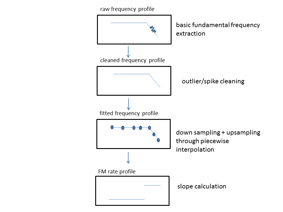
CF-FM segmentation occurs through a multi step process. First the instantaneous frequency of the signal is estimated at a sample-level resolution, the raw frequency profile - raw_fp. Then the raw_fp is refined as it can be quite noisy because of well, noise, or abrupt changes in signal level across the sound.

Minor jumps will be corrected to give rise to the cleaned frequency profile - cleaned_fp. The cleaned_fp however, is a very high-resolution look into the sound’s frequency profile. Even though the temporal resolution is high, the spectral resolution is limited by the size of the pwvd_window (refer to the original docs here). This limited spectral resolution means each sample will not have a unique value. For instance if the frequency of sound is increasing linearly with time, the cleaned_fp may actually look like steps going up. These ‘steps’ cause issues while calculating the rate of frequency modulation - fmrate, and so , the cleaned_fp is actually downsampled and then upsampled by interpolation. This gives rise to the fitted frequency profile - fitted_fp.

The fitted_fp captures the local trends and doesn’t have the step like nature of cleaned_fp. If we were to actually measure frequency modulation from cleaned_fp there’d be lots of 0 modulation regions and many very brief bursts of FM regions wherever a ‘step’ rose or dropped. Thanks to the sample-wise unique values in fitted_fp we can now calculate the local variation in frequency modulation across the sound.

Let’s now check the frequency profiles once more

out_refined_inspector.visualise_frequency_profiles()

Out:

(<AxesSubplot:xlabel='Time, s', ylabel='Frequency, Hz'>, <AxesSubplot:>)

The raw and cleaned frequency profiles are very similar, though the ‘cleanliness’ in the cleaned_fp is visible especially because the frequency profile doesn’ wildly jump around towards the end of the call. The fitted_fp also closely matches the cleaned_fp though it seems to rise later and drop faster. This is because of the downsampling that happens to estimate the fmrate. The rise time is a direct indicator of the downsampling factor, which samples the cleaned_fp at periodic intervals, and is thus called sample_every. The sample_every parameter defaults to 1% of the input signal duration. If the frequency profiles broadly match the actual call as seen coarsely on a spectrogram.

Step 2: Check the fmrate profile

CF and FM parts of a call are segmented based on the rate of frequency modulation they show. The fmrate is a np.array with the estimated frequency modulation rate in kHz/ms. Yes, pay attention to the units, it’s not kHz/s, but kHz/ms! Let’s take a look at the FM rate profile for this sound.

out_refined_inspector.visualise_fmrate()

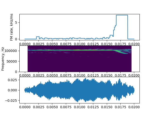
Out:

(<AxesSubplot:ylabel='FM rate, kHz/ms'>, <AxesSubplot:xlabel='Time, s', ylabel='Frequency, Hz'>, <AxesSubplot:>)

Let’s compare this fmrate profile with the final CF-FM segmentation.

out_refined_inspector.visualise_cffm_segmentation()

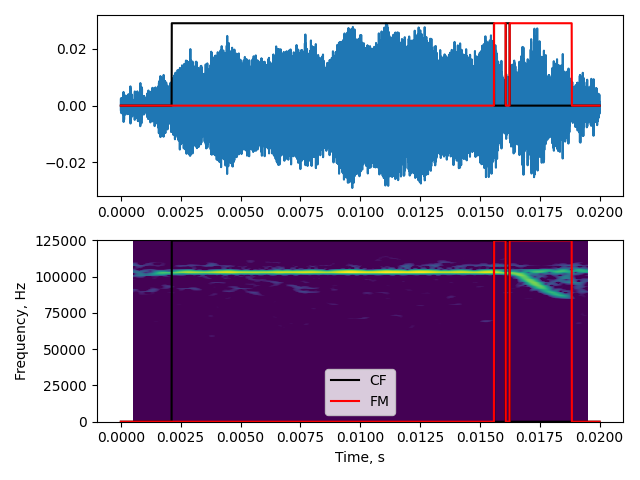
Out:

(<AxesSubplot:>, <AxesSubplot:xlabel='Time, s', ylabel='Frequency, Hz'>)

Something’s odd – even though the FM rate seems to be close to zero near the actual FM parts, parts of it are still being classified as FM!! What’s happening. Let’s take a closer look at the FM rate profile, but zoom in so the y-axis is more limited. Let’s also overlay the CF-FM segmentation results over this.

seg_out, call_parts, msmts = outputs_refined
cf, fm, info = seg_out

w,s,a = out_refined_inspector.visualise_fmrate()
w.set_ylim(0,5)
t_min, t_max = 0.01, 0.02
w.set_xlim(t_min, t_max)
s.set_xlim(t_min, t_max)
a.set_xlim(t_min, t_max)
w.plot()
itsfm.make_waveform(cf*4,fs)
itsfm.make_waveform(fm*4,fs)
plt.tight_layout()

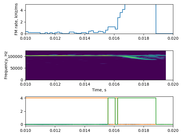
From this you can clearly see that the FM part correspond to tiny peaks in the fmrate which reach around 1 kHz/ms. It may of course be no surprise once you know the default fmrate_threshold is 1 kHz/ms. This rate doesn’ make sense for bat call FM portions as they have much high frequency modulation rates. The easy way to estimate the relevant fmrate_threshold is to eyeball the start and end frequencies of a call part and calculate the fm rate!

Step 3: Set a relevant fmrate_threshold

For this example call any FM rate above 0.5kHz/ms will allow a sensible segmentation of the CF and FM parts. Lets set it more conservatively at 2kHz/ms, this will reduce false positives. In general, for this particular call type, the FM sweep has an approximate rate of 5-6kHz/ms, and so we should definitely be able to pick up the FM region with a threshold of 2kHz/ms.

# add an additional keyword argument
keywords['fmrate_threshold'] = 2.0 # kHz/ms

output_newfmr = itsfm.segment_and_measure_call(audio, fs,**keywords)

out_newfmr_insp = itsfm.itsFMInspector(output_newfmr, audio, fs)
out_newfmr_insp.visualise_cffm_segmentation()

Out:

(<AxesSubplot:>, <AxesSubplot:xlabel='Time, s', ylabel='Frequency, Hz'>)

Summary

This tutorial exposed some of the messy details behind the PWVD frequency tracking. In most cases, I hope you won’t need to think so much about the parameter choices. However, some basic playing around will definitely be necessary each time you’re handling a new type of sound or recording type. Hopefully, this has either allowed you to get a glimpse into the system. Do let me know if there’s something (or everythin) is confusing, and not clear!