Bat call example

The <INSERTNEWNAME> package has many example recordings of bat calls thanks to the generous contributions of bioacousticians around the world:

import matplotlib.pyplot as plt
import numpy as np
import itsfm
from itsfm.run_example_analysis import contributors
print(contributors)

Out:

Cannot import SoundFile!!
/home/docs/checkouts/readthedocs.org/user_builds/itsfm/envs/latest/lib/python3.7/site-packages/itsfm-0.0.1-py3.7.egg/itsfm/data/__init__.py:17: UserWarning:

 The package soundfile could not be imported properly. Check your installation.Using the scipy.io package for now.
  warnings.warn(msg1+msg2)
/home/docs/checkouts/readthedocs.org/user_builds/itsfm/envs/latest/lib/python3.7/site-packages/itsfm-0.0.1-py3.7.egg/itsfm/data/__init__.py:66: WavFileWarning: Chunk (non-data) not understood, skipping it.
  fs_original, audio = wav.read(each)
/home/docs/checkouts/readthedocs.org/user_builds/itsfm/envs/latest/lib/python3.7/site-packages/itsfm-0.0.1-py3.7.egg/itsfm
/home/docs/checkouts/readthedocs.org/user_builds/itsfm/envs/latest/lib/python3.7/site-packages/itsfm-0.0.1-py3.7.egg/itsfm/data_contributors.csv
0          Aditya Krishna
1              Aiqing Lin
2    Klaus-Gerhard Heller
3              Neetash MR
4         Laura Stidsholt
Name: people, dtype: object

from itsfm.data import example_calls, all_wav_files

Separating the constant frequency (CF) and frequency-modulated parts of a call

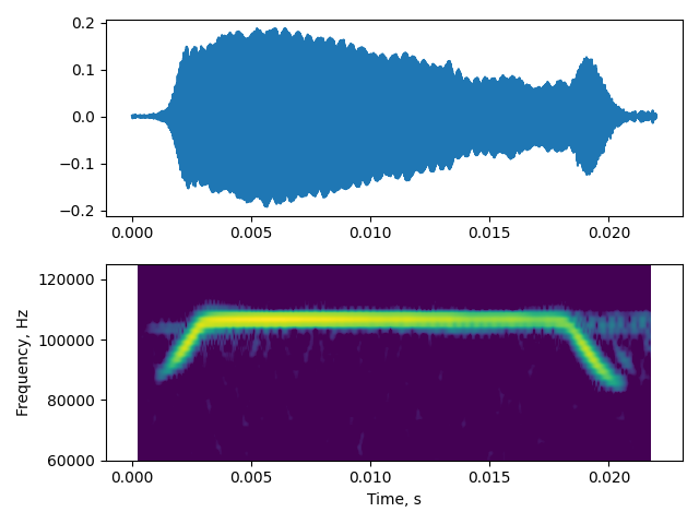
Here, let’s take an example R. mehelyi/euryale(?) call recording. These bats emit what are called ‘CF-FM’ calls. This is what it looks like.

bat_rec = list(map( lambda X: '2018-08-17_34_134' in X, all_wav_files))
index = bat_rec.index(True)
audio, fs = example_calls[index] # load the relevant example audio

w,s = itsfm.visualise_sound(audio,fs, fft_size=128)
# set the ylim of the spectrogram narrow to check out the call in more detail
s.set_ylim(60000, 125000)

Out:

(60000.0, 125000.0)

Now, let’s segment and get some basic measurements from this call. Ignore the actual parameter settings for now. We’ll ease into it later !

non_default_parameters = {
                          'segment_method':'pwvd',
                          'signal_level':-26, # dBrms re 1
                          'fmrate_threshold':2.0, # kHz/ms
                          'max_acc':2.0, # kHz/ms^2
                          'window_size':int(fs*0.0015) # number of samples
                          }
outputs = itsfm.segment_and_measure_call(audio, fs,
                                        **non_default_parameters)

# load the results into a convenience class
# itsFMinspector parses the output and creates diagnostic plots
# and access to the underlying diagnostic data itself

output_inspect = itsfm.itsFMInspector(outputs, audio, fs)

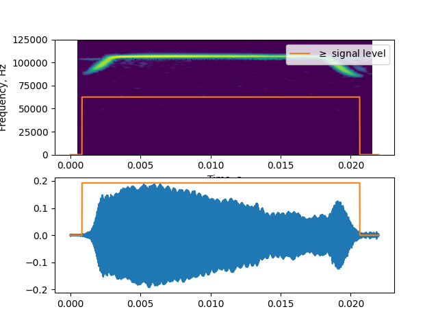
Let’s check that the threshold we chose actually matches the region of audio we’re interested in

output_inspect.visualise_geq_signallevel()

Out:

(<AxesSubplot:xlabel='Time, s', ylabel='Frequency, Hz'>, <AxesSubplot:>)

Let’s take a look at how long the different parts of the call are.

output_inspect.measurements

Verifying the CF-FM segmentations

Here, let’s see where the calls are in time and how they match the spectrogram output

output_inspect.visualise_cffm_segmentation()
plt.tight_layout()
plt.savefig('pwvd_cffm_segmentation.png')

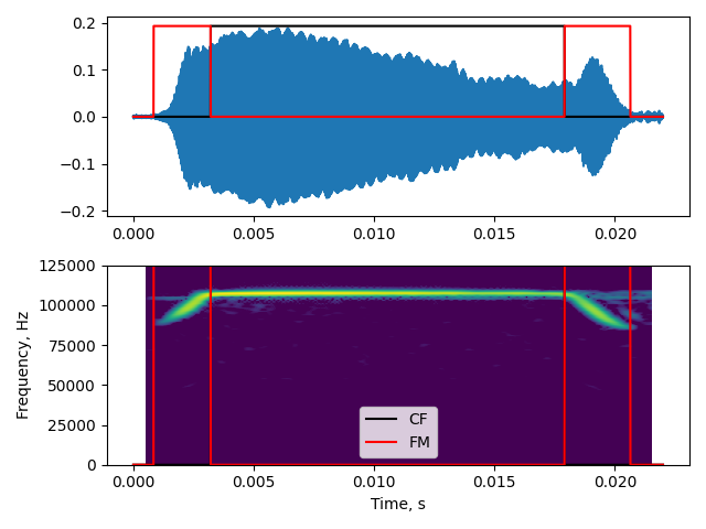
Even without understanding what’s happening here, you can see the ‘sloped’ regions are within the red boxes, and the ‘relatively even region is in the black box. These are the FM and CF parts of this call.

The underlying frequency profile of a sound

The CF and FM parts of a call in the ‘pwvd’ method is based on actually tracking the instantaneous frequency of the call with high temporal resolution. With this profile, the rate of frequency change, or modulation can be calculated for each region. Using a threshold rate of the frequency modulation, call regions above and below it can be easily identified!

s,w = output_inspect.visualise_frequency_profiles()
s.legend_.remove()

handles, labels = s.get_legend_handles_labels()
labels_new = ['Raw frequency profile (FP)','Error corrected FP','Downsampled FP']
l = s.legend(handles, labels_new, loc=8, fontsize=11,
               borderaxespad=0., frameon=False, labelcolor='w')
s.set_ylabel('Frequency, Hz', labelpad=-1.5)
plt.savefig('pwvd_freqprofiles.png')

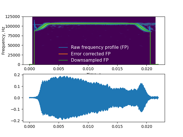
You can see from the plot above that the frequency profile of the sound shows a relatively constant frequency region of the call in middle and with frequency modulated regions in the middle.

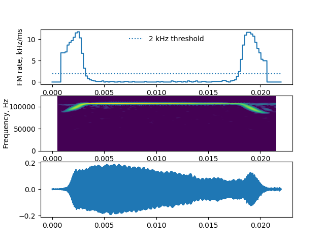
The underlying frequency modulation rate

fmrate_plot, spec, waveform = output_inspect.visualise_fmrate()
fmrate_plot.hlines(2,0,audio.size/fs, linestyle='dotted',label='2 kHz threshold')
fmrate_plot.legend(frameon=False)
plt.savefig('pwvd_fmrate_diagnostic.png')

Performing measurements on the CF and FM parts of a call

We were just able to get some measurements on the Cf and FM parts of the call. What if we want more information, eg. the rms, and peak frequency of each CF and FM call part? This is where <insertname> has a bunch of inbuilt and customisable measurement functions.

inbuilt_measures = [itsfm.measure_peak_frequency,
                       itsfm.measure_rms]

non_default_parameters['measurements'] = inbuilt_measures

The output is a tuple with 3 objects in it related to the segmentation individual call parts and the measurements made on them. We’re happy with the actual segmentation, and so won’ be making anymore diagnostic plots, and won’ need to call itsFMInspector anymore. We can unpack the outputs into its components and just view the measurements.

seg_out, call_parts, results_inbuilt = itsfm.segment_and_measure_call(audio, fs,
                                             **non_default_parameters
                                                 )
results_inbuilt

The results are output as a pandas DataFrame, which means they can be easily saved as a csv file if you were to run it in your system. Each row corresponds to one identified CF or FM region in an audio recording.

Defining custom measurements

If the inbuilt measurement functions are not enough - then you may want to write your own. See the documentation for what a measurement function must look like by typing help(itsfm.measurement_function). The ‘peak_to_peak’ function below calculates the difference between the highest negative and highest positive value. This effectively the maximum range of values that the signal takes.

def peak_to_peak(whole_audio, fs, segment, **kwargs):
    '''
    Calculates the range between the minimum and the maximum of the audio
    samples.
    '''
    relevant_audio = whole_audio[segment]
    peak2peak = np.max(relevant_audio) - np.min(relevant_audio)
    return {'peak2peak':peak2peak}

custom_measure_fn = [peak_to_peak]

# add the custom_measure list to the :code:`non_default_parameters` dictionary
#
non_default_parameters['measurements'] = custom_measure_fn



seg_out, call_parts, results_custom = itsfm.segment_and_measure_call(audio, fs,
                                                                   **non_default_parameters
                                                 )
results_custom

Of course, needless to say, you can also mix and match inbuilt with custom defined measurement functions.

mixed_measures = [peak_to_peak, itsfm.measure_rms]
non_default_parameters['measurements'] = mixed_measures

seg_out, call_parts, results_mixed = itsfm.segment_and_measure_call(audio, fs,
                                             **non_default_parameters
                                                 )
results_mixed