The peak-percentage method

The peak percentage method works if the constant frequency portion of a sound segment is the highest frequency. For instance, in CF-FM bat calls, the calls typically have a CF and one or two FM segments connected.

This method is loosely based on the spectrogram based CF-FM segmentation in [1], but most importantly it differs because it is implemented completely in the time-domain.

How does it work?

A constant frequency segment in any sound leads to a peak in the power spectrum. The same audio is high-passed and low-passed at a threshold frequency that’s very close (eg. 99% of the peak frequency)

and just below the peak frequency. This creates two versions of the same sound, one with an emphasis on the CF, and one with the emphasis on

the FM. By comparing the two sounds, the segmentation proceeds to detect CF and FM parts.

References

[1]Schoeppler, D., Schnitzler, H. U., & Denzinger, A. (2018). Precise Doppler shift compensation in the hipposiderid bat,

Hipposideros armiger. Scientific reports, 8(1), 1-11.

import matplotlib.pyplot as plt
import scipy.signal as signal
import itsfm
from itsfm.simulate_calls import make_cffm_call
from itsfm.segment import segment_call_into_cf_fm

from itsfm.data import example_calls, all_wav_files

bat_rec = list(map( lambda X: '2018-08-17_34_134' in X, all_wav_files))
index = bat_rec.index(True)
audio, fs = example_calls[index] # load the relevant example audio

w,s = itsfm.visualise_sound(audio,fs, fft_size=128)
# set the ylim of the spectrogram narrow to check out the call in more detail
s.set_ylim(60000, 125000)

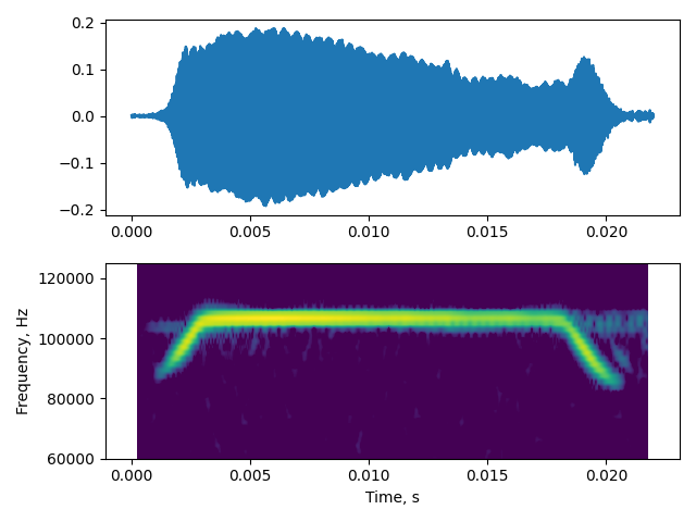
Out:

(60000.0, 125000.0)

Now, let’s proceed to run the peak-percentage based segmentation.

non_default_params = {'segment_method':'peak_percentage',
                      'window_size':int(fs*0.0015),
                      'signal_level':-30,
                      'double_pass':True}
outputs = itsfm.segment_and_measure_call(audio, fs,
                                        **non_default_params)

# load the results into a convenience class
# itsFMinspector parses the output and creates diagnostic plots
# and access to the underlying diagnostic data itself

output_inspect = itsfm.itsFMInspector(outputs, audio, fs)

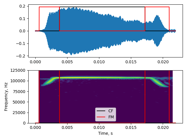
Verifying the CF-FM segmentations

Here, let’s see what the output of the peak-percentage method shows

output_inspect.visualise_cffm_segmentation()
plt.tight_layout()
plt.savefig('pwvd_cffm_segmentation.png')

Low/high passed audio profiles

Let’s also take a look at the low and high -passed audio profiles. The regions where the dB rms of the high-passed audio is greater than the low-passed audio is considered CF and vice-versa is considered FM.

spec, profiles = output_inspect.visualise_pkpctage_profiles()
profiles.legend(loc=9, frameon=False)
plt.savefig('pkpctage_profiles.png')

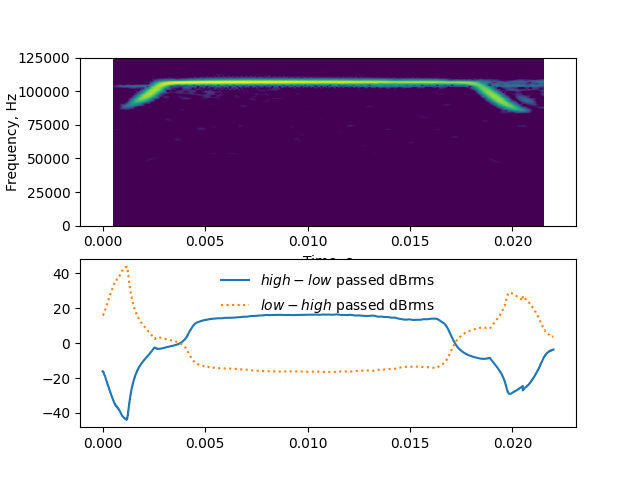
The two profiles match the expected CF/FM regions fairly well.