Segmenting with the PWVD method

The ‘PWVD’ method stands for the Pseudo Wigner-Ville Distribution. It is a class of time-frequency representations that can be used to be gain very high spectro- temporal resolution of a sound [1,2], and can outdo the spectrogram in terms of how well it allows the tracking of frequency over time.

How does it work?

The PWVD is made by performing a local auto-correlation at each sample in the audio signal, with a window applied onto it later. The FFT of this windowed- auto correlation reveals the local spectro-temporal content. However, because of the fact that there are so many auto-correlations and FFT’s involved in its construction - the PWVD can therefore take much more time to generate.

Note

The ‘tftb’ package [3] is used to generate the PWVD representation in this package. The website is also a great place to see more examples and great graphics of the PWVD and alternate time-frequency distributions!.

References

[1] Cohen, L. (1995). Time-frequency analysis (Vol. 778). Prentice hall.

[2] Boashash, B. (2015). Time-frequency signal analysis and processing: a comprehensive reference. Academic Press.

[3] Jaidev Deshpande, tftb 0.1.1, https://tftb.readthedocs.io/en/latest/auto_examples/index.html

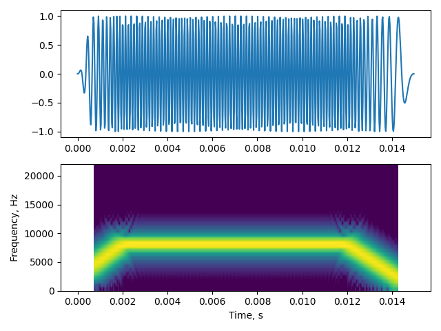
Let’s begin by making a synthetic CF-FM call which looks a lot like a horseshoe/leaf nosed bat’s call

import matplotlib.pyplot as plt
import numpy as np
import scipy.signal as signal
import itsfm
from itsfm.frequency_tracking import generate_pwvd_frequency_profile
from itsfm.frequency_tracking import pwvd_transform
from itsfm.simulate_calls import make_cffm_call
from itsfm.segment import segment_call_into_cf_fm

fs = 44100
call_props = {'cf':(8000, 0.01),
                     'upfm':(2000,0.002),
                     'downfm':(100,0.003)}

cffm_call, freq_profile = make_cffm_call(call_props, fs)
cffm_call *= signal.tukey(cffm_call.size, 0.1)

w,s = itsfm.visualise_sound(cffm_call, fs, fft_size=64)

The PWVD is a somewhat new representation to most people, so let’s just check out an example

pwvd = pwvd_transform(cffm_call, fs)

The output is an NsamplesxNsamples matrix, where Nsamples is the number of samples in the original audio.

plt.figure()
plt.imshow(abs(pwvd), origin='lower')
num_rows = pwvd.shape[0]
plt.yticks(np.linspace(0,num_rows,11), np.linspace(0, fs*0.5, 11))
plt.ylabel('Frequency, Hz')
plt.xticks(np.linspace(0,num_rows,5),
           np.round(np.linspace(0, cffm_call.size/fs, 5),3))
plt.xlabel('Time,seconds')

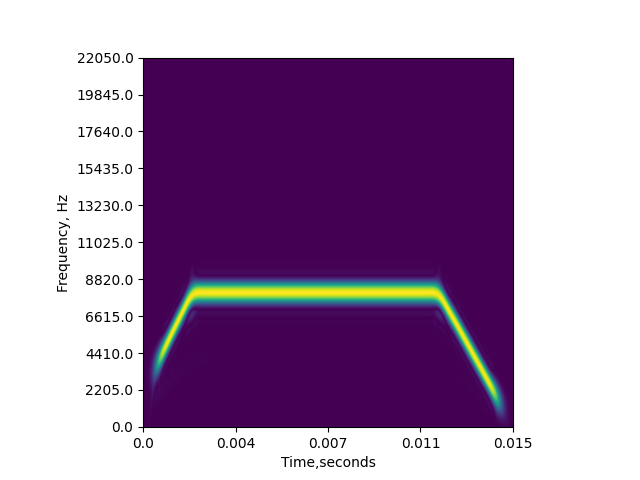
Out:

Text(0.5, 0, 'Time,seconds')

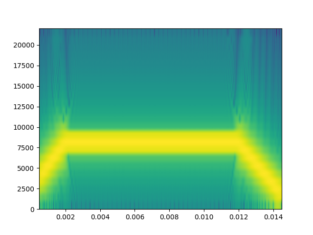
In comparison to the ‘crisp’ time-frequency representation of the PWVD, let’s compare how a spectrogram with comparable parameters looks:

onems_samples = int(fs*0.001)
plt.figure()
out = plt.specgram(cffm_call, Fs=fs, NFFT=onems_samples, noverlap=onems_samples-1)

The dominant frequency at each sample can be tracked to see how the the frequency changes over time. Let’s not get into the details right away, and proceed with the segmentation first.

cf, fm, info = segment_call_into_cf_fm(cffm_call, fs, segment_method='pwvd',
                                                                            window_size=50)

The segment_call_into_cf_fm provides the estimates of which samples are CF and FM. The info object is a dictionary with content that varies according to the segmentation method used. For instance:

info.keys()

Out:

dict_keys(['moving_dbrms', 'geq_signal_level', 'raw_fp', 'acc_profile', 'spikey_regions', 'fmrate', 'cleaned_fp', 'fitted_fp'])